Essential Math For Understanding Neural Networks

Hello fellow human, I hope I can help you with your journey in learning machine learning. This should cover essential math for neural networks. We go through: partial derivatives, multidimensional graphs, scalars, vectors, matrices, tensors, and few most important distributions in probability. For all listed topics, I will present an example in machine learning and how it is applied. To make a note, I will not explain concepts behind neural networks in this article; I intend to make your learning experience of NN more comfortable to digest by having the necessary knowledge of mathematics, which are applied in algorithms at the rear of NN or at least guide you in the right direction.

Let’s start with the basics of partial derivatives. They are common in machine learning, especially in backpropagation which is used to adjust weights in neural networks. We use partial derivatives in backpropagation to determine how specific weights or biases affect the loss function. Notation for differentiating partial derivatives from ordinary derivatives is a very artistic d symbol, ∂.

Let’s say we have a multivariable function:

Computing partial derivative with respect to x would look like this:

When we are calculating expression above, we are looking at y and z as constants.

We know if we have ordinary derivative df/dx in a single variable calculus, what that says is: for a tiny change in x, how much will output of a function change. But how can we interpret that if we have a multivariable function f(x,y) = x²y ? A dx still represents a tiny change in input variable x, and df can for sure still represent resulting change of the function. But x is not the only direction in which we can move, we are also in multidimensional space, we can move in y-direction too. Now we can calculate df/dy and that tells us how does the output change for a small shift in the y-direction. We can conclude that neither of those two derivatives tells us the full story of how does the function change, that is the reason we call them partial derivatives. This is how a two variable function would look in 3d space:

The more formal definition of single-variable derivative is this:

If we choose two values of some function f(x₀) and f(x₁) and want to calculate slope of secant between them, we would do so by using rise over run formula.

Now we know, if distance between f(x₀) and f(x₁) gets really small we would get slope of a tangent in value f(x₀). If we rewrite that formula with delta x representing some small nudge, we get:

But we can not just put delta x as zero because we would get 0/0, and that is undefined form, also that is the reason we need to use limit as delta x approaches zeros, but is never zero. So when we calculate derivative of a function at some point we get the slope of a tangent at that point. For partial derivative with respect to x, the formal definition is really similar:

Important to notice that delta x noted as tiny input is added to different input variables depending on partial derivative we are taking. But what is the graphical explanation when we calculate the partial derivative of an multivariable function. If we imagine we have two variable function f(x,y)=…, and calculate partial derivative with respect to x in some specific point, we can visualize that by drawing plane across graph as constant y-value and measuring the slope of resulting cut. For great visualization, I refer you to this video.

One more aspect of partial derivatives is the multivariable chain rule, which is used in backpropagation. I will present you with the basics to start understanding it. Single-variable chain rule states that the derivative of an composite function f(g(x)) is f’(g(x))*g’(x). Now let’s look at the example:

Deriving this function would look like this:

What we actually did was this:

Now looking at multivariable chain rule should be easier, and it is used in equation* below.

In neural networks, it arises when we try to calculate the partial derivative of a function with respect to some variable, but that variable depends on variables before it. In the context of backpropagation, a partial derivative of the cost of the function C with respect to weight in the lᵗʰ layer that connects kᵗʰ neuron with jᵗʰ neuron would look like this(“a” represents mᵗʰ neuron in Lᵗʰ layer):

*Partial derivative of a cost function with respect to weight

Now to better explain and visualize the equation above, we will define what gradient descent is. The gradient of a function is a way of grouping all partial derivatives of a function. Let’s say we have this function: f(x,y)=x²sin(y). Partial derivative with respect to x is:

and partial derivative with respect to y is:

Now we denote gradient of a function f with symbol nabla:

We can call this function a vector-valued function that takes as an input two-dimensional point and outputs a two-dimensional vector. If we did this with four-dimensional input, we would get four-dimensional output. A useful way of looking at gradient is as an operator which form is vector full of partial derivatives with respect to different variables( in machine learning that number can be few millions) that we can multiple with a function, and we can see how would we get the format I have written above.

A gradient of a function is the path of the steepest ascent, in geometrical interpretation, what path we need to take so we reach a local maximum in the least number of steps. So now that we know what gradient is, it is easier to define gradient descent, and that is the path of the steepest descent and we get it by taking steps proportional to negative of the gradient, in other words, the way of finding local minimum as a method of minimizing a loss function. I would recommend you to check out Khan Academy website for more information on partial derivatives and multivariable calculus, and 3Blue1Brown Youtube channel. For more information about backpropagation and detailed explanation check out this book.

We have to include parts of linear algebra in our journey, all data points in a neural network are in the form of tensors and that makes it highly efficient in a coding environment to write and for computing units to calculate. Datasets, images are all in matrix form, each row has the same length, i.e the same number of columns, therefore we can say that the data is vectorized and each row represents specific data input. Rows can be provided to the model one at the time or in a batch. Let’s start with scalars. A scalar is just a single number and when we define it, it will be noted as n∈R where n is the slope of the line for example.A vector is an array of numbers, we can think of each number in vector as a number defining coordinate along a different axis.

The first element of x is x₁, the second x₂… If we also want to say what kind of numbers are stored in vector x, i.e if each element is real number, and the vector has n elements, then the vector lies in the set formed by taking the Cartesian product (Cartesian product of two sets A and B is denoted by A x B and defined as: A×B = { (a,b) | aϵA and bϵB }) of ℝ n times, ℝⁿ. A matrix is a 2-D array of numbers, so each element is identified by two indices instead of just one, but in neural networks, we need X-D array and they are called tensors. Let’s say we have a tensor named A and we want to identify the element of A at coordinates (i,j,k) by writing Aᵢⱼₖ.An important operation on matrices is the transpose, which is a mirror image of matrix across a diagonal line, called the main diagonal. It runs from the upper left corner down and right. We denote the transpose of a matrix A as A^T, defined such that:

We can add matrices together, as long as they have the same shape just by adding their corresponding elements C = A+B where Cᵢⱼ=Aᵢⱼ+Bᵢⱼ. We can add a scalar to the matrix or multiply by a scalar only by performing that operation on each element of a matrix. In the notation that is more popular when working with neural networks, we allow the addition of a matrix and a vector, that will give us another matrix: C = A + b, where Cᵢⱼ=Aᵢⱼ+Bⱼ. In other words, the vector b is added to each row of the matrix. That way, we do not need to define a matrix with “b” that is copied into each row before doing the addition.

The most operations in neural networks are the multiplications of two matrices. The matrix product of two matrices A and B is the third matrix C. The rule is that matrix A must have the same number of columns as matrix B has rows. If the shape of matrix A is k x n and B is n x g, then the shape of matrix C is k x g. The product operation is defined by:

If you want to know more, please refer to mathematics literature or this book.

Now we will go through a few concepts from probability that are common in machine learning.

Mean squared error is a statistical method that measures the average squared difference between the estimated value and what is estimated, in machine learning, we use it as a loss function, furthermore to find out how much our guesses are wrong from labeled data.

If we imagine our yᵢ as results (predicted data by our NN) that are scattered on a two-dimensional graph as points and yᵢ’ as labeled data that lies on a line that follows the best-scattered data put differently minimizes the error, our goal is to find that line y=Mx+B. Simply put; after every batch, we calculate mean squared error and try to minimize it in the next one and our goal, of course, is to make it the closest possible to zero meaning our predicted points are the closest possible to line y = Mx+B.

Another popular method for evaluating loss is Cross-Entropy, which is a measure of the difference between two probability distributions for a given random variable or set of events. It outputs a probability value between 0 and 1, and increases as the predicted probability diverge from the labeled data. We can calculate loss using this formula, where p(x) is the target probability, and q(x) is the predicted probability.

If the last layer with softmax activation function outputs these probabilities for given classes:

and our data in one-hot encoding for that specific training example is:

As we can see out predicted distribution is different from labeled values and we want to calculate that difference, we would do so by using Cross-Entropy and then nudge weights and biases of the NN, so we minimize that difference. Preceding summation operator in the Cross-Entropy formula above we had to put minus because logarithmic function outputs negative values for inputs that are less than 1 and that is always the case here because we are dealing with probabilities which softmax function outputs.

Now let’s list some activation functions and their graphs. The main reason we are not using linear functions as activation functions is that we can not use backpropagation to train a model. The derivative of linear function is constant and has no relation to the input. That is the reason we use non-linear functions. I will list a couple of them but I will no go into depth, nor go through pros and cons; for that, I refer you to this article.The Sigmoid function. The range of a Sigmoid function is <0,1>.

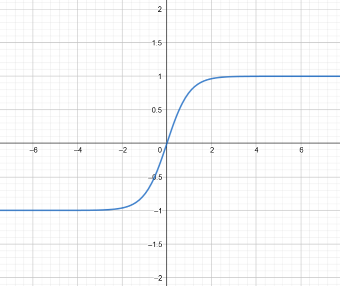
The TanH ( Hyperbolic Tangent) function. The range of a TanH is [-1, 1].

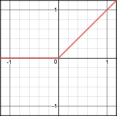
The ReLU function which stands for Rectified Linear Units, the formula is really simple max(0,x), it is similar to Sigmoid function but avoids vanishing gradient problem.

In this article we went through a few most used mathematical concepts in machine learning, briefly explained them and linked literature for more information on specific topics. There is still a lot of stuff I have not mentioned, but I hope this can be a good starting point for your journey or just a good memory refresh. Thank you for reading.